Relationship between acoustic indices, length of recordings and processing time: a methodological test

Introduction

Quantifying biological diversity is fundamental for setting priorities for conservation (Brooks et al., 2006; Mittermeier et al., 1998), particularly in the current period of dramatic biodiversity loss (Ceballos et al., 2015). This has traditionally relied on detailed species inventories, which often demands an intense, costly sampling effort, especially in high-biodiversity areas (Lawton et al., 1998). Funding constraints mean many countries have been unable to implement adequate monitoring and therefore lack vital biodiversity information (Collen et al., 2008), and there is an urgent need to develop more efficient monitoring strategies. One approach has been to develop rapid biodiversity assessment methods that obtain indicators from indirect cues of diversity, such as the sound produced by animals (Sueur et al., 2008).

Examining the spatial and temporal variation in, and relationships between, sounds that emerge from biological, geophysical and anthropogenic sources to form a “soundscape” can provide fundamental insights into environmental patterns and processes operating across landscapes (Pijanowski et al., 2011; Sueur & Farina, 2015). Whilst the use of acoustic tools in biodiversity conservation is not new (Baptista & Gaunt, 1997), its use as a tool for monitoring biodiversity health and quantifying responses to land-use change and management has grown rapidly in recent years (Ritts et al., 2016). It is particularly valuable in ecological research and conservation biology, because it is non-invasive, sensitive to multiple taxa, and allows widespread data collection since several places can be simultaneously surveyed (Gasc et al., 2015; Machado et al., 2017).

Analytical tools for processing soundscape recordings have improved in recent years, enabling large amounts of data to be readily analysed with minimal acoustical expertise through the use of standardised acoustic indices (Gasc et al., 2015). These acoustic indices can be used to quantify, for example, the acoustic complexity, diversity or evenness of a soundscape at a specific place during a limited time period (Gasc et al., 2013). Given that the biophony - sounds generated by the community of species present - is a major contributor to soundscapes, the potential for using acoustic indices for biodiversity monitoring has been explored using both computational experiments (Zhao et al., 2019) and by evaluating their correlation with field-derived measurements such as number of song types (Sueur et al., 2008), species richness (Jorge et al., 2018; Towsey et al., 2014), and functional diversity (Gasc et al., 2013). Indeed, acoustic analyses are now widely used for biodiversity monitoring and methodological guidelines for sampling design (Sugai et al., 2019), which recommend the use of continuous recordings and the selection of a range of acoustic indices to better capture site variability and acoustic complexity, have recently been developed (Bradfer-Lawrence et al., 2019). However, meeting these guidelines requires the collection and storage of large data files and can pose significant data processing challenges that remain to be explored. Furthermore, there are still unresolved questions around how acoustic indices represent different elements of biodiversity and how to optimize their use for acoustic monitoring and their relationship with sampling schedule and recording duration.

The present study focuses on the behaviour of acoustic indices according to recording duration and sampling regularity, in order to inform the optimal sampling strategy for biodiversity assessments; shorter and less frequent recordings result in a slower drain of recording device batteries and reduced storage requirements, thus allowing devices to be deployed for longer periods of time, but may not capture fine-scale temporal variation in acoustic characteristics. We also calculated the processing time required to undertake each acoustic analysis. Specifically, we test the performance of and required processing time for five different acoustic indices (Acoustic Complexity Index (ACI) (Pieretti et al., 2011); Acoustic Diversity Index (ADI) (Villanueva-Rivera et al., 2011); Acoustic Evenness Index (AEI) (Villanueva-Rivera et al., 2011); Acoustic Entropy Index (H) (Sueur et al., 2008); and Normalized Difference Soundscape Index (NDSI) (Kasten et al., 2012), using recordings varying in length from 1 minute to 60 minutes and collected in the mega diverse settings of the Brazilian Amazon and Cerrado.

Material and methods

Study area. Sound files were recorded in two locations in Brazil: Site 1 (0°01’08.0”S-51°07’22.1”W) is a secondary Amazon rainforest patch surrounded by farms and minor urban areas, whilst Site 2 (21°42’51.3”S-45°00’42.4”W) is three kilometres away from an urban area and located in a secondary forest of transition between Mata Atlantica and Cerrado.

Data collection. SongMeter SM4 © recorders (Wildlife Acoustics, Inc.) were used to record sounds in both sampling sites in January 2018. The devices were programmed to continuously record one-hour WAV files at the default settings (i. e. 24 kHz sampling rate, 16 bits, stereo), for a total of 88 hours in site 1 and 50 hours in site 2. Each one-hour file was 345.3 MB and all 138 files together sum 47.7 GB. However, 44 files were subsequently discarded due to loud geophysical sounds (e.g. rain, thunder) that masked sounds from other sources (Sánchez-Giraldo et al., 2020). This selection was done by checking spectrograms made with Kaleidoscope software version 4.5.4 (Wildlife Acoustics Inc, 2017).

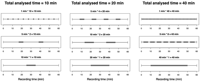
Subsampling. To analyse the influence of recording duration on acoustic index characteristics, each of the 94 one-hour recordings was split into consecutive length class subsamples of 1, 5, 10, 15, 20, 30 and 40 minutes, resulting in 60 subsamples of 1 minute, 12 of 5 minutes, 6 of 10 minutes, 4 of 15 minutes, 3 of 20 minutes, 2 of 30 minutes and 1 of 40 minutes per original recording. The 40-minute subsample was taken from between minutes 10 and 50 of the original recording. To evaluate the appropriate number of subsamples to take (hereafter subsample frequency), we compared the performance of acoustic indices derived from continuous blocks of recording, with those derived from recordings representing the same total duration, but comprising multiple, shorter recordings spread evenly across the full-hour recording period. For example, acoustic indices for 40 subsamples of 1 minute, 8 of 5 minutes, 4 of 10 minutes, 2 of 20 minutes and 1 of 40 minutes were compared (Figure 1).

Figure 1: Experimental design examples for different combinations of subsample frequency, adding up to a total analysed time of 10, 20 and 40 minutes. Grey segments represent the subsamples taken from one-hour files.

Data processing. All statistical and sound analyses were performed using R software version 3.4.3 (R Core Team, 2018) and the soundecology package (Villanueva-Rivera & Pijanowski, 2016), with ACI, ADI, AEI, H and NDSI calculated using default parameters in the multiple sounds function. Since ACI is a cumulative index, it was divided by the length in minutes of each subsample to get a comparable range of values, as recommended in soundecology package description; other indices had no further calculations.

Statistical analysis. Spearman Rank correlations were performed to test for associations between the five indices and, for each index in turn, between the value derived from processing the complete one-hour recording and those from processing subsamples of varying duration. For the subsample frequency analysis, index values derived from all subsamples present in a specific combination of frequency and recording duration (Figure 1) were averaged, and this value was then correlated with the index value derived from processing the complete one-hour recording they were subsampled from.

Processing time. Processing time was defined as the time taken to calculate each acoustic index for a given recording and is expected to vary according to computing capabilities. This study was performed in two phases, each with different computing capabilities.

Phase 1 was a preliminary analysis, for which calculations were run on a computer with an Intel Core i7 processor running at 1.8 GHz, using 4GB 1333 MHz DDR3 of RAM, running Mac OS X 10.8 Mountain Lion. Phase 2 was run in a more powerful computer with an Intel Core i7 processor running at 3.2 GHz, using 64GB 2667 MHz DDR4 of RAM, running macOS 10.14 Mojave. Note that, ACI can only be calculated for recordings up to about 20 minutes; in phase 1, a simple linear regression was used to predict processing time for recordings of 30, 40 and 60 minutes, but in phase 2, ACI processing times for 30, 40 and 60 minutes were obtained by summing index values derived from the appropriate number of 10-minute recordings.

Results

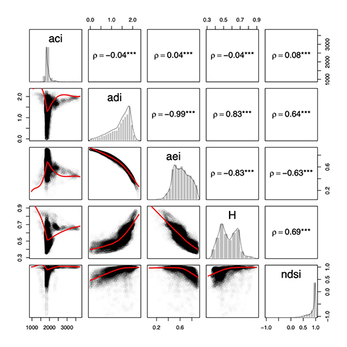
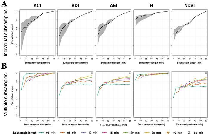
Acoustic Complexity Index (ACI). Whilst statistically significant, the correlations between ACI and the other acoustic indices were weakest, with no clear linear patterns identified (Figure 2). Reducing recording length introduced most variation in ACI, with correlation values for indices for individual 1-minute samples and their associated one-hour recording varying between 0.55 and 0.87, with a median of 0.76 (Figure 3A). As subsample duration increased, median correlation values increased and the range of correlation values for individual subsamples of the same duration decreased, with the level of the lowest correlation values increasing quicker than that of the highest correlation value (Figure 3A). Splitting the total sampling period into multiple, shorter sampling periods of the same total length improved sample representativeness (Figure 3B). This is especially noticeable for shorter subsamples, with the average metric across 10 or more one-minute subsamples having a correlation values with the index from the associated one-hour recording of >0.97 (Figure 3B).

Figure 2: Data distribution and associations between acoustic indices. Spearman correlation values and scatterplots between indices (n = 42 864), and histograms with a density line for each index are shown. Red line indicates a LOESS (locally estimated scatterplot smoothing). All correlations have p-values less than 0.001 (‘***’). ACI-Acoustic Complexity Index, ADI- Acoustic Diversity Index, AEI-Acoustic Evenness Index, H-Acoustic Entropy Index and NDMS-Normalized Difference Soundscape Index

Figure 3: Spearman rank correlation between: A, the acoustic index value for each subsample duration and the complete one-hour recording from which it was subsampled; B, mean index values for subsamples representing combinations of recording length and subsample frequency (see Methods and Figure 1 for more details) and the complete one-hour recording. In A, the black line indicates the median of correlation values and the shaded areas denote the range. ACI,Acoustic Complexity Index; ADI, Acoustic Diversity Index; AEI, Acoustic Evenness Index; H,Acoustic Entropy Index; NDSI,Normalized Difference Soundscape Index.

Acoustic Diversity Index (ADI) and Acoustic Evenness Index (AEI). Although ADI and AEI measure different acoustic characteristics (Villanueva-Rivera et al., 2011), they were very strongly and negatively correlated (Spearman ρ = -0.99, n = 42 864, p < 0.001, Figure 2). As subsample duration increased, so the strength of the correlation between the ADI for the subsample and ADI for the associated one-hour recording also increased, with variability in correlation strength between individual subsamples of the same duration and the full recording also decreasing. A similar pattern was evident for AEI (Figure 3A). Continuous recordings were more representative of the associated one-hour recording than recordings of the same total duration, but split over multiple, shorter subsamples (Figure 3B). Interestingly, index values averaged over multiple subsamples were never truly representative of the full hour recording, even if the cumulative time sampled was very high. For instance, averaged ADI values for 60 1-minute subsamples had the same degree of correlation (0.88) with the whole hour as the averaged ADI values for 10 1-minute subsamples (Figure 3B).

Acoustic Entropy (H). H showed a strong positive correlation with ADI and NDSI, a strong negative correlation with AEI, and a very weak but significant negative correlation with ACI (Figure 2). Among all indices, H showed the highest correlation between values for subsamples and full recordings and lowest variability between subsamples of the same duration (Figure 3A). Half of the correlations between 1-minute subsamples and their associated one-hour recording were above 0.9, with the lowest correlation value was 0.72 (Figure 3A). H follows a similar pattern to ACI in that index values averaged across multiple, shorter samples were more representative of the one-hour recording than values from a continuous recording of the same total length (Figure 3B). That is, for example, the average index value for 10 samples of 1-minute was more strongly correlated with the index value for the associated one-hour recording than the average metric across 2 samples of 5 minutes or the metric for one 10-minute sample (Figure 3B).

Normalized Difference Soundscape Index (NDSI). This index is weakly associated with the other indices calculated in this study (Figure 2) but shows similar patterns to ADI and AEI with regard recording length and subsampling frequency (Figure 3). NDSI was the most sensitive index to recording length, showing the sharpest decline in correlation values when shortening subsample length (Figure 3A). However, the variability in correlation strength between individual sub-samples of the same length and the associated one-hour recording was lower than for the other indices examined, particularly at shorter subsample lengths (Figure 3A). As with ADI and AEI, index values from continuous recordings tended to be more representative of the one-hour recordings than averaged values from across multiple, shorter subsamples of the same total length (Figure 3B).

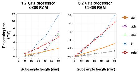
Processing time. Processing time for all indices increased with increasing recording length, but the rate of increase differed between indices. Both absolute time and rate of increase was substantially lower with increased computational capabilities. For short-duration recordings, or with high computing capabilities (3.2 GHz processor and 64GB RAM), ADI, AEI and ACI processing times were approximately one-third to one-quarter those of H and NDSI but, at lower computing capabilities (1.7 GHz processor and 4GB RAM), processing time for ADI and AEI increased exponentially with increasing recording duration and exceeding NDSI processing time for 60-minute recordings (Figure 4).

Figure 4: Mean processing time for computing acoustic indices at each recording length with two different equipments, using the multiple_sounds function in soundecology R package (Villanueva-Rivera & Pijanowski, 2016). Standard error bars are not shown as they were negligible, due to consistency in processing time (mean relative standard error of 0.28%).

Total processing time was 195.9 hours, equivalent to ~8 days, using high computing capabilities for calculating five acoustic indices to all subsamples and the complete one-hour file (i.e. 120.9 hours of subsamples divided in: 391 of 1 minute, 78 of 5 minutes, 21 of 10 minutes, 10 of 15 minutes, 6 of 20 minutes, 3 of 30 minutes, 1 of 40 minutes and 1 of 60 minutes). Total processing time for each index was 28.1 hours for ACI, 13.5 hours for ADI, 13.5 hours for AEI, 64.0 hours for H and 76.8 hours for NDSI.

Discussion

Studies into the use of acoustic indices in environmental research suggest that continuous recordings in the field are preferable, because they might reduce the deployment times required to capture soundscape variability (Bradfer-Lawrence et al., 2019). However, we show that distributing samples of shorter recording length across the survey period (i.e., representative of the population of continuous recordings) can offer an opportunity to optimize data collection and processing, while identifying analogous patterns in acoustic indices values, much more for ACI and H than for AEI, ADI or NDSI. Given that recommendations for acoustic monitoring suggest collecting a minimum of 120 hours of audio recordings per site to reduce acoustic indices variability and improve precision (Bradfer-Lawrence et al., 2019), such targeted subsampling could greatly reduce data storage and computational power requirements.

Index choice, frequency of recording and optimal recording length will all depend on the biodiversity characteristics being inferred from soundscape records. For example, NDSI is highly informative in measuring changes of anthropogenic pressures, as it gives an indication of an increase (or decrease) in anthrophony (Kasten et al., 2012), whilst ACI, ADI, AEI, and H are more related to direct diversity measures (e.g.Bradfer-Lawrence et al., 2019; Gasc et al., 2013; Jorge et al., 2018; Sueur et al., 2008; Towsey et al., 2014). Whilst indices derived from shorter recordings are broadly representative of the immediate time period from which they are sampled, our results do suggest that both the precision and accuracy of ACI, ADI and AEI in particular will decrease with recording duration (Figure 3A). However, NDSI precision seems less affected by recording duration, whilst the precision and accuracy of H appear more stable under changes in recording duration. Each acoustic index also behaves differently in response to changes in sampling frequency, with measures of AEI, ADI and NDSI more robust under continuous recording formats and ACI and H more robust under shorter, more frequent recording formats.

Although index choice should primarily be determined by the research objectives, other considerations, such as processing time, might help in the index selection, especially if computational power is a limiting factor. When computational capability is limited, calculation time of H from short recordings is equivalent to that for other indices, but as recording length increases, processing times for H increase exponentially and the calculation time of H from a one-hour recording is twice that required for other indices. This could be related to the way it is computed, as it is estimated as the product of both temporal and a spectral entropy, which requires the computation of a mean spectrum using a Short Time Fourier Transform based on a non-overlapping sliding function window (Sueur et al., 2008). If focusing on acoustic characteristics represented by H, it would be much more efficient to use multiple shorter recording lengths, especially as the index value itself seems robust to this type of recording schedule. ADI and AEI processing time also increased exponentially with recording duration, but only with low computational capabilities. This is likely to be related to computer memory saturation and reduction of processing performance. Conversely, NDSI and ACI present a linear trend for both computational capabilities, probably explained by their simpler calculation that involves few steps, and their relative slow rate of increase in processing time with increasing recording duration makes them valuable indices when dealing with large amounts of data (Pieretti et al., 2011). Index computation optimization can also be achieved by evaluating the correlation between indices before conducting further processing and analysis; ADI, AEI and H appear highly correlated so computing all of them may be redundant as they reflect the same acoustic patterns.

When designing a recording schedule for biodiversity assessments using acoustic information, it is important to consider how the acoustic index behaves in relation to the duration and periodicity of samples. Long term projects for monitoring changes in biodiversity may prefer to use shorter recordings to prolong sampling periods and capture a wider temporal space. In such cases, we recommend the use of ACI and H, due to their accuracy and precision to representing soundscape characteristics with short recordings. Additionally, data processing would be less demanding (in particular for big data analysis), thus enabling rapid assessments and on-time actions to changes under the scope of biodiversity conservation.